Outlier audits

Utility bills can sometimes be too high, or too low, or just not what you were expecting. Outlier audits help flag unusual bills by comparing them against past trends.

To do this, we use a bit of math: quadratic equations and R² (R squared).

Why use a quadratic equation?

We want to see how things like energy use, cost, or demand change depending on the average daily temperature (avgMDT).

How bills are flagged

After all the calculations for each bill are complete (see steps below), the system assigns an adjusted z-score to the bill. This score shows how much the bill differs from expected values and determines whether it's an outlier.

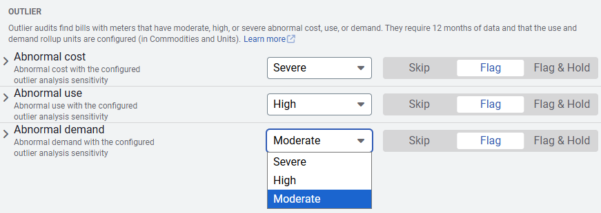
Bills marked as outliers are categorized as severe, high, or moderate, based on the score.

You can control when bills are flagged in the Audits screen, located in the Bills module menu. From there, select the desired outlier level to decide which bills are flagged for review.

The math basics (explained simply)

Quadratic equation

A quadratic equation looks like this:

y = ax² + bx + c

The graph makes a U-shape curve (up or down).
In this case:
- x = average daily temperature
- y = use/day, cost/day, or demand

Why a curve? Because energy use doesn't always change in a straight line. For example:

Cold → high heating costs
Warm → low heating costs
Hot → high cooling costs

What is R²?

R² (R squared) is a number between 0 and 1.
It shows how well the curve matches reality.
- 1.0 (or close) → Perfect fit. The model (curve) explains almost all variation.
- 0.0 (or close) → Bad fit. The model doesn't explain much.

👉In other words: Higher R² = more trust in the model.

How the outlier audit works

Collect history
• Takes the last 12-24 non-void bills.
• Needs at least 12 bills to build the model (curve) to make a prediction.
Fit curves for three things
For each bill, EnergyCAP fits quadratic equations (curved line) against average daily temperature (avgMDT = (High Temp + Low Temp) ÷ 2), because energy use often bends up/down with hot and cold weather.

Fit means: EnergyCAP tries to draw a curved line through the cloud of data points (temperature vs bill value). It adjusts a, b, c so that the curve is as close as possible to the actual historical data.

Makes three quadratic curves: Use per day, Cost per day, and Demand

EnergyCAP records for each bill:
• Predicted value (from the curve)
• Residual = Actual - Predicted
• R² = How well the curve explains history (0 = bad, 1 = perfect)

Standardize the differences (z-score style)
For the current bill:
• If the standard deviation is 0, set z = 0.
• Positive z: actual bill is higher than the model.
• Negative z: actual bill is lower than the model.
Apply the R² offset to get an adjusted z-score
The model is trusted more if R² is high. So we make outliers harder to trigger based on the R² value. The R² value determines how much of an offset is added or subtracted to the original z-score.
* See below for the details of how the offset is applied.

Why adjust a z-score with an R² offset?
The adjustment is about balancing statistical math with practical trust in the model. EnergyCAP adds or subtracts an offset based on the R² to tune the severity.
• The z-score alone tells you how unusual the bill is compared to historical variation.
• But if the model (the curve) doesn't fit very well (low R²) then the z-score might not mean much
• If the model does fit history very well (high R²), then we should trust the z-score more and therefore flag outliers more aggressively.
Map adjusted z-score to a severity level
Severity is how "bad" the outlier looks.
* See severity levels below.
Audits use severity levels
In EnergyCAP audit settings, you can select what bills you want flagged, SEVERE, HIGH, or MODERATE
• An adjusted z-score of 1 → only SEVERE
• An adjusted z-score of 2 → SEVERE + HIGH
• An adjusted z-score of 3 → SEVERE + HIGH + MODERATE

Quick cheat sheet (used in every example)

Diff (residual) = Actual − Predicted
z-score = Diff ÷ StdDev (how unusual the bill is)
Offset from R² (how strict we are):
- R² ≥ 0.97 → 8
- R² ≥ 0.95 → 5
- R² ≥ 0.90 → 3
- R² ≥ 0.85 → 1
- R² < 0.85 → 0
Adjust z with offset
- If Diff > 0 (positive): z_adj = z − offset
- If Diff < 0 (negative): z_adj = z + offset
Severity
- Positive side:
  - ≥ 3.0 → SEVERE (1)
  - ≥ 2.0 → HIGH (2)
  - ≥ 1.5 → MODERATE (3)
  - else → None (4)
- Negative side:
  - ≤ −5.0 → SEVERE (1)
  - ≤ −4.0 → HIGH (2)
  - ≤ −3.0 → MODERATE (3)
  - else → None (4)

Example A — SEVERE (1) (Use per day, positive residual)

Setup

Predicted: 100.0
Actual: 106.2
StdDev: 1.0
R²: 0.90 → offset 3

Steps

Diff = 106.2 − 100.0 = +6.2
z = 6.2 ÷ 1.0 = 6.2
Positive branch → z_adj = 6.2 − 3 = 3.2
3.2 ≥ 3.0 → SEVERE (1)

Why? Big positive miss and a pretty good model (R² 0.90) → it’s flagged hard.

Example B — HIGH (2) (Direct cost per day, negative residual)

Setup

Predicted: 200.0
Actual: 154.0
StdDev: 5.0
R²: 0.95 → offset 5

Steps

Diff = 154.0 − 200.0 = −46.0
z = −46.0 ÷ 5.0 = −9.2
Negative branch → z_adj = −9.2 + 5 = −4.2
−5.0 < −4.2 ≤ −4.0 → HIGH (2)

Why? Very low actual vs predicted, but the strict offset softened it from Severe to High.

Example C — MODERATE (3) (Demand, positive residual)

Setup

Predicted: 150.0
Actual: 152.8
StdDev: 1.0
R²: 0.86 → offset 1

Steps

Diff = 152.8 − 150.0 = +2.8
z = 2.8 ÷ 1.0 = 2.8
Positive branch → z_adj = 2.8 − 1 = 1.8
1.5 ≤ 1.8 < 2.0 → MODERATE (3)

Why? It’s above expected, but the model isn’t super tight, so it lands at Moderate.

Example D — HIGH (2) (“Low Fit” R²)

Setup

Predicted: 120.0
Actual: 123.0
StdDev: 1.5
R²: 0.40 → offset 0

Steps

Diff = 123.0 − 120.0 = +3.0
z = 3.0 ÷ 1.5 = 2.0
Positive branch → z_adj = 2.0 − 0 = 2.0
2.0 ≤ z_adj < 3.0 → HIGH (2)

Why? Even with a loose model (low R², no offset), the difference is still big enough to be “High.”